Read AlexNet, VGG, GoogLeNet and ResNet as four fixes to four failures

By 2012 the ImageNet challenge had stalled at hand-engineered features, and the four designs that broke the stall are the reference points worth reading closely. Read them in order, because the order is the argument: each one is the previous design's measured failure, answered with a concrete change — to training, to depth, to budget, to wiring — never a new kind of layer.

flowchart LR
  IM[ImageNet] --> AN[AlexNet: trains]
  AN --> VG[VGG: deeper]
  VG --> GN[GoogLeNet: cheaper]
  GN --> RN[ResNet: trainable depth]

One rule governs the order: every design answers the previous one's measured failure — training (AlexNet), depth (VGG), cost (GoogLeNet), depth that trains (ResNet).

1 · The scoreboard

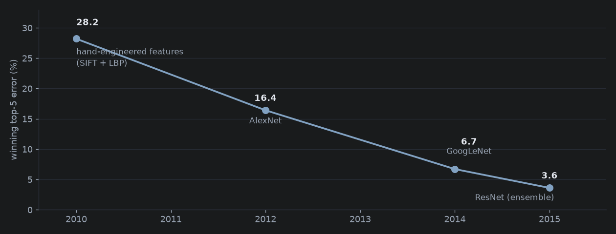
The ImageNet challenge (ILSVRC) gave every entrant one job: put an image into one of 1000 classes. The training set held 1,281,167 labeled images. The score was top-5 error — the fraction of test images whose true class is missing from the model's five best guesses. A model that guesses five classes at random covers the truth 5/1000 of the time, so it lands near 99.5% error; the numbers below are earned, not lucky. In 2010 and 2011 the winners used hand-engineered features (SIFT, LBP, Fisher vectors); the 2010 winner scored 28.2%, so the right class was missing from more than one image in four.

2 · The words this page uses

Seven groups of words carry the rest of the page. Read them once. Each one comes back with a number later.

2.1 · Top-5 error

A classifier writes one score per class. Top-5 error is the fraction of test images whose true class is not among the five highest scores. A model that puts the right class in second place still counts as correct. Top-1 error is the stricter count: the fraction whose best guess is wrong. With 1,000 classes, five distinct random guesses contain the truth \(\frac{5}{1000}\) of the time, so random guessing scores 99.5% top-5 error.

2.2 · Parameter, parameter budget, depth

A parameter is one number training can change: one weight or one bias. The parameter budget is the total count and how it splits between the convolution layers and the head. At four bytes per number, one million parameters take 4 MB, and the budget decides whether the model fits the card. Depth counts the layers that carry a weight matrix: convolutions and fully connected layers. BatchNorm carries two numbers per channel, and a pool, a ReLU or a dropout carries none, so none of those add to depth. AlexNet is 8 layers deep (5 conv, 3 fully connected), VGG16 is 16 (13 conv, 3 fully connected), and ResNet-34 is 34 (33 conv, 1 fully connected).

2.3 · Kernel, filter, channel depth, head

A kernel is the small grid of weights a convolution slides over its input: a 3×3 kernel has nine weights per input channel. A filter is one kernel across all input channels, plus one bias, and it writes one output channel. The number of input channels is also called the channel depth. So a 3×3 filter on a 96-channel input holds \(3 \times 3 \times 96 = 864\) weights. The head is the part after the last feature map: a flatten or a global average pool, then the fully connected layers that write the class scores.

2.4 · Receptive field

The receptive field of one output cell is the patch of the input that can change its value. A single 3×3 convolution sees 3×3. A second 3×3 convolution reads 3×3 cells of the first, and each of those already saw 3×3, so the second sees 5×5 of the input. Each extra 3×3 layer adds one pixel of reach on every side: \(n\) layers see \((2n+1) \times (2n+1)\).

2.5 · Block, stage, stride

A block is a short fixed sequence of layers repeated with the same shape rule: VGG's block is two or three 3×3 convolutions, then a pool. A stage is a group of blocks with one channel count and one map size; the next stage starts where the map halves and the channels double. Stride is how far a kernel moves per step: stride 1 with padding 1 keeps the size, stride 2 halves it.

2.6 · Residual and shortcut

A shortcut, also called a skip connection, is a wire that carries a block's input past the block and adds it to the block's output. The residual is what the block's layers learn instead of the whole mapping: \(F(x) = H(x) - x\), the change from the input. The block returns \(H(x) = F(x) + x\). Set every weight in \(F\) to zero and the block returns \(x\) unchanged, so doing nothing is free to represent.

2.7 · Bottleneck and 1×1 convolution

A 1×1 convolution reads one pixel across all input channels and writes one number per output channel. It mixes channels, not space, so its cost does not grow with the image size. A bottleneck is a narrow layer between two wide ones. GoogLeNet puts a 1×1 conv in front of each 3×3 and 5×5 branch to squeeze the channel count before the expensive kernel. ResNet-50's block is 1×1 down, 3×3, 1×1 up, so the 3×3 works on a quarter of the channels.

3 · AlexNet: make a deep net train

AlexNet (Krizhevsky, Sutskever and Hinton, 2012) bet that the convolution was already enough — the problem was getting a deep stack of them to train on this data at all. Its shape, in the single-card view this page uses:

Every size comes from \(\frac{H - K}{S} + 1\): \(\frac{227 - 11}{4} + 1 = 55\), then the pools give 55 → 27 → 13 → 6. (The paper's text says 224; its figure and this arithmetic say 227 — the stride-4 math lands on 55 only with 227.) The paper splits the model over two GPUs, so its conv2 reads 5×5×48; one card holding all channels reads 5×5×96.

Two numbers set a layer's weight count: filter count and input depth. conv1: \(96 \times 11 \times 11 \times 3 = 34{,}848\). conv2: \(256 \times 5 \times 5 \times 96 = 614{,}400\) — the 256 filters each span all 96 input channels. The same rule, summed over the five conv layers, and the head, flattened from \(6 \times 6 \times 256 = 9216\):

def conv_w(filters, k, c_in):
    return filters * k * k * c_in + filters     # weights + one bias per filter

convs = [(96, 11, 3), (256, 5, 96), (384, 3, 256), (384, 3, 384), (256, 3, 384)]
conv_total = sum(conv_w(f, k, c) for f, k, c in convs)          # 3,747,200
head_total = (9216*4096 + 4096) + (4096*4096 + 4096) + (4096*1000 + 1000)
print(conv_total, head_total)                                   # 3747200 58631144

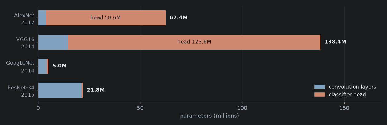
Run it. Both numbers then reappear in every count below — and in the figure's first bar.

The shape of the bill is the surprise: the head holds 94% of the weights, and fc1 alone \((9216 \times 4096 = 37.7M)\) outweighs all five conv layers ten to one. The paper rounds the total to “60 million”. Where the 62M sit — and where they sit in the three designs that follow — is the next figure.

Three choices made this stack train. ReLU replaced sigmoid: a sigmoid's gradient collapses to near zero once it saturates, and a deep stack multiplies those small numbers together, while ReLU passes the gradient through unchanged for positive inputs. Dropout 0.5 landed in the head — where 94% of the weights live — zeroing half the units each step so none can lean on its neighbors. Two GTX 580s: the model and its activations did not fit one 3GB card, so it was split across two. The run itself: about 90 passes over the 1.2M-image training set, five to six days.

Result: 16.4% top-5, against the runner-up's 26.2%. The winning error had fallen by more than a third in one entry — with the same convolution as everyone else.

4 · VGG: deepen one block

VGG (Simonyan and Zisserman, 2014) pushed one idea as far as it goes: deeper, with nothing new. One block, repeated. The block is a 3×3 convolution with padding 1 (size holds), then ReLU — stacked two or three times — then 2×2 max pool, which halves both spatial dims. Channels double at every pool: 64, 64 → 128, 128 → 256, 256, 256 → 512 ×3 → 512 ×3. That is 13 conv layers, then AlexNet's kind of head: flatten \(7 \times 7 \times 512 = 25{,}088\), then 4096, 4096, 1000.

Why 3×3 everywhere, never a big kernel? Same field of view, fewer multiplies. A pair of stacked 3×3 convs reaches a 5×5 patch — the second layer reads 3×3 positions of the first, and each of those already read 3×3 — at \(2 \times 9 = 18\) multiplies per output position, against 25 for one 5×5. Three stacked 3×3 convs reach 7×7 at 27 against 49. The pair is 28% cheaper, the triple 45%, and each extra layer adds a fresh ReLU that one big conv cannot. With \(C\) input and output channels both sides scale by \(C^2\) (\(18C^2\) against \(25C^2\)), and every choice runs over every output position — so input size cancels out of the comparison.

The doubling is the second half of the discipline. A pool keeps one of every four positions; doubling both channel counts multiplies the work per position by four. Positions divide by four as work multiplies by four — each layer's total multiply count stays roughly flat while the information moves up into channels.

All the size lands in the head: \(25{,}088 \times 4096 = 102{,}760{,}448\) weights in one layer, 1.6× AlexNet's entire network; the three head layers hold 123,642,856 of VGG16's 138,357,544 total, while all 13 conv layers hold 14,714,688. Nearly nine tenths of VGG16 is a classifier bolted onto the convs — the second bar of the figure above.

Result: 7.3% top-5 for the 19-layer version, second to GoogLeNet's 6.7%, at 19.6 billion multiply-adds per image. Better than AlexNet by a wide margin — but the machine grew 2.2× in weights, and the head grew with it. VGG's durable lesson is the block: small kernels, uniform, repeated. The head had to go.

5 · GoogLeNet: cheaper depth

GoogLeNet (Szegedy and colleagues, 2014) answered VGG's bill with two structural moves: compute several scales at once in every module, and delete the fully connected head.

5.1 · The inception module

Four branches run on the same input: a bare 1×1 conv; 1×1 then 3×3; 1×1 then 5×5; a 3×3 max pool then 1×1. The branches merge by concatenating their output channels — stacked, not added. Addition is elementwise: it needs equal shapes, and it forces the same channel slot to mean the same thing in every branch. The branches answer different-scale questions, so their answers stay separate, and the next layer learns how much to trust each group.

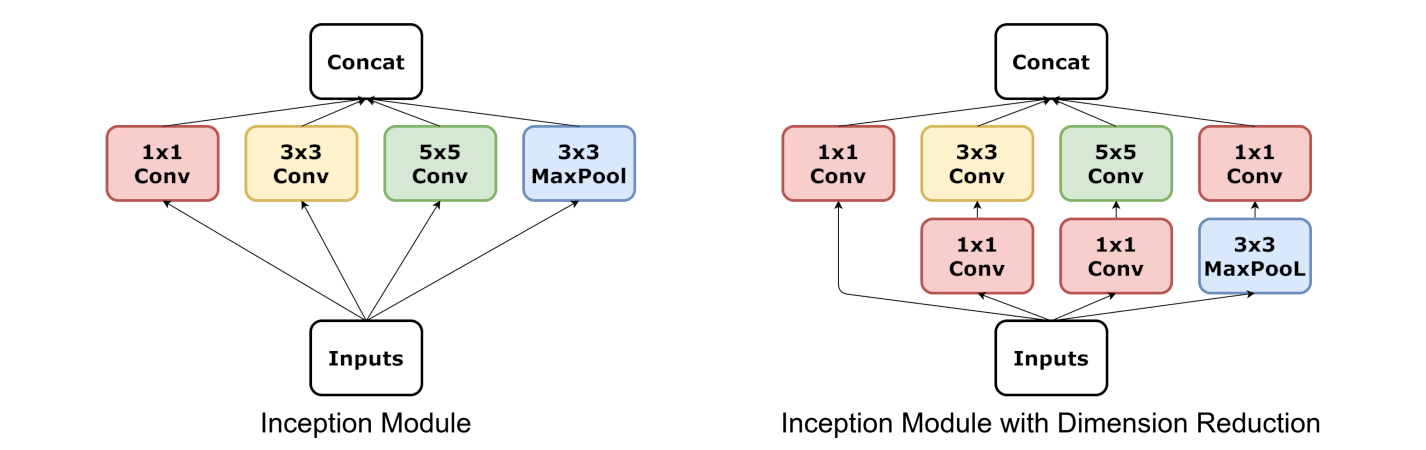
The 1×1 convs in front of the 3×3 and 5×5 branches are the cost trick. A 5×5 conv reading 512 channels and writing 64 multiplies \(512 \times 64 \times 25 = 819{,}200\) values per output position. Squeeze the input to 64 channels first — \(512 \times 64 = 32{,}768\) — and the 5×5 now reads 64 channels: \(64 \times 64 \times 25 = 102{,}400\). Total 135,168: about 6× fewer multiplies, plus a free extra ReLU. A 1×1 conv reads one pixel across all channels — a learned cross-channel mix, no spatial mixing — which is exactly the projection the branch needs.

5.2 · The head, deleted

After the modules the net holds 1024 maps of 7×7. Flatten-and-FC would cost \(7 \times 7 \times 1024 \times 1000 = 50{,}176{,}000\) weights. Instead each map is averaged to a single number — global average pooling — and one linear layer classifies 1024 numbers: \(1024 \times 1000 = 1{,}024{,}000\) weights. The head shrinks 49×. With no giant FC the whole network fits in about 6.8M parameters, roughly a tenth of AlexNet's 62.4M and a twentieth of VGG16's 138.4M. The paper's own headline is 12× fewer than AlexNet — the 5.0M bar in the figure. The 5.0M is that rounded claim; the 6.8M is the count usually quoted for the 22-layer net. Both are small next to VGG.

Result: 22 weight layers, 6.67% top-5 — the 2014 win — with VGG second at 7.3%. Nearly the same error as VGG at a fraction of the size: depth stopped being a weight-count competition.

6 · ResNet: depth that trains

ResNet (He and colleagues, 2015) started from an anomaly. When plain conv nets get deeper, error gets worse — and the training error gets worse, not only the test error.

Read what that rules out. A 56-layer net contains its 20-layer sibling: keep the 20 layers, and let all 36 extra layers compute the identity — a deeper model's solution space includes every shallower solution, and more. And training error is fit to data the model is being trained on, so a model with more capacity fitting worse is not overfitting. One reading is left: optimization fails to reach solutions that demonstrably exist.

The fix is one line of wiring: \(H(x) = F(x) + x\). The conv stack no longer learns the whole mapping \(H\); it learns the change \(F\) — the residual — and a shortcut adds the input \(x\) back. Identity becomes free: drive \(F\)'s weights to zero and \(H(x) = x\) falls out. The exact behavior a deeper plain net keeps failing to learn costs nothing to specify here.

Two more properties fall out of the same add. Backward: \(\frac{\partial H}{\partial x}\) contains the identity term, so gradient arriving at the block reaches \(x\) — and everything before it — without passing through a weight; a stack of convs can shrink a signal, the shortcut carries it undamaged. Forward: addition is elementwise, so \(F(x)\) and \(x\) must match in shape. Inside a stage, stride 1 with padding 1 keeps every block shape-preserving and the raw input is added. At a stage boundary the main path halves the map (stride 2) and doubles the channels; there the shortcut becomes a 1×1 conv with stride 2 — the dotted shortcut in the paper's figures.

flowchart LR
  X[x] --> C1[3x3 conv]
  C1 --> R1[ReLU]
  R1 --> C2[3x3 conv]
  X --> ADD[add]
  C2 --> ADD
  ADD --> R2[ReLU]

What one block computes: \(H(x) = F(x) + x\). The stack makes the change; the shortcut carries the input around it; the add needs matching shapes.

The template, 34-layer version: 7×7 stride-2 conv to 64 channels; 3×3 stride-2 max pool; then stages of residual blocks — 3 blocks at 64 channels, 4 at 128, 6 at 256, 3 at 512 — where the first block of each stage strides 2 to halve the map; then global average pooling and a 1000-way linear layer. Downsizing is the striders' job; within a stage every block is shape-preserving, so the raw shortcut works everywhere inside.

Count it: 21,276,160 weights in the convolutions, 513,000 in the final linear layer — 21,789,160 total, against VGG16's 138,357,544. The 34-layer net is deeper than VGG19's 19 weight layers, 6.4× smaller in parameters, 5.4× cheaper in multiply-adds (3.6B against 19.6B) — and more accurate: an ensemble of 152-layer ResNets won ILSVRC-2015 at 3.57% top-5. Depth was trainable.

The 50-layer version swaps each two-conv block for a bottleneck — 1×1 down, 3×3, 1×1 up — and holds 25.6M parameters, still under a fifth of VGG16. Half again the depth costs about 17% more parameters than the 34-layer net's 21.8M.

7 · The arithmetic on one layer

One rule prices a convolution layer. One shape check decides whether an add runs. Both fit on a line, and every convolution count on the page comes from them.

7.1 · What one convolution layer costs

A convolution layer with a \(k \times k\) kernel, \(C_{\mathrm{in}}\) input channels and \(C_{\mathrm{out}}\) filters holds \[ k \times k \times C_{\mathrm{in}} \times C_{\mathrm{out}} + C_{\mathrm{out}} \] parameters. The product counts the weights. Each of the \(C_{\mathrm{out}}\) filters spans all \(C_{\mathrm{in}}\) input channels, and each channel contributes a \(k \times k\) patch. The last term is one bias per filter.

AlexNet's conv3 reads 256 channels and writes 384 with a 3×3 kernel: \[ 3 \times 3 \times 256 \times 384 = 884{,}736 \] weights, plus 384 biases, for 885,120 parameters. VGG16's 3×3 layers at 256 channels read 256 and write 256: \[ 3 \times 3 \times 256 \times 256 = 589{,}824 \] weights, plus 256 biases, for 590,080 parameters.

AlexNet's conv1 is \(11 \times 11 \times 3 \times 96 + 96 = 34{,}944\), cheap because it reads only three colour channels. Channel depth multiplies the price: VGG's 256→256 layer costs about 17× that, and its 512→512 layers cost about 68×.

7.2 · The 1×1 bottleneck's saving

Take a 5×5 branch that reads 512 channels and writes 64. Without a projection, one output position costs \(5 \times 5 \times 512 \times 64 = 819{,}200\) multiplies. With a 1×1 conv in front that writes 64 channels first, the projection costs \[ 512 \times 64 = 32{,}768 \] multiplies, and the 5×5 then reads 64 channels: \[ 5 \times 5 \times 64 \times 64 = 102{,}400. \] Together that is \(32{,}768 + 102{,}400 = 135{,}168\). The saving is \(819{,}200 - 135{,}168 = 684{,}032\), a factor of \(\frac{819{,}200}{135{,}168} = 6.06\). The 1×1 layer pays 32,768 multiplies of its own and adds a ReLU. The 5×5 now reads a learned 64-channel summary instead of the raw 512, so the saving is real but the summary can lose information.

7.3 · The residual add's shape rule

Addition is elementwise, so \(F(x)\) and \(x\) must have the same batch, channels, height and width. Inside a stage nothing moves: a 3×3 conv with padding 1 and stride 1 keeps 56×56, the channel count stays 64, and a (2, 64, 56, 56) input adds to a (2, 64, 56, 56) block output. Each side holds \(2 \times 64 \times 56 \times 56 = 401{,}408\) numbers.

At a stage boundary the main path strides 2 and doubles the channels: the block writes (2, 128, 28, 28), with \(2 \times 128 \times 28 \times 28 = 200{,}704\) numbers, while the shortcut still carries (2, 64, 56, 56). Both the channel count and the two sides differ, so the add fails. The fix is the dotted shortcut in the paper's figure: a 1×1 conv with stride 2 that maps 64 channels at 56×56 to 128 at 28×28. It holds \(1 \times 1 \times 64 \times 128 + 128 = 8{,}320\) parameters.

8 · Run it: shapes and counts

Every output below comes from the CPU build of PyTorch. Write your prediction before you run a block; the comment on the print line is the output to expect.

8.1 · Count a 3×3 layer

Predict first. nn.Conv2d(256, 256, 3, padding=1) makes one 3×3 layer from 256 channels to 256. How many parameters does it hold, and what is the weight tensor's shape?

import torch.nn as nn

layer = nn.Conv2d(256, 256, 3, padding=1)
print(layer.weight.shape)                          # torch.Size([256, 256, 3, 3])
print(layer.bias.shape)                            # torch.Size([256])
print(sum(p.numel() for p in layer.parameters()))  # 590080

What happens. The count is 589,824 weights plus 256 biases, the 590,080 of §7.1. The weight shape reads (out, in, kernel height, kernel width): 256 filters, each 256×3×3. The layer's parameter count does not depend on the image size; only the number of positions it runs over does.

8.2 · A residual block keeps its shape

Predict first. The block below is the one from §6: two 3×3 convs at 64 channels, a BatchNorm after each, and the input added to the second conv's output. Feed it a (2, 64, 56, 56) batch. What shape comes out, and how many parameters does the block hold?

import torch, torch.nn as nn

class Block(nn.Module):
    def __init__(self, ch):
        super().__init__()
        self.c1 = nn.Conv2d(ch, ch, 3, padding=1, bias=False)
        self.b1 = nn.BatchNorm2d(ch)
        self.c2 = nn.Conv2d(ch, ch, 3, padding=1, bias=False)
        self.b2 = nn.BatchNorm2d(ch)
        self.relu = nn.ReLU(inplace=True)

    def forward(self, x):
        out = self.relu(self.b1(self.c1(x)))
        out = self.b2(self.c2(out))
        return self.relu(out + x)          # the add needs x and out to match

block = Block(64)
x = torch.zeros(2, 64, 56, 56)
print(block(x).shape)                      # torch.Size([2, 64, 56, 56])
print(sum(p.numel() for p in block.parameters()))   # 73984

What happens. The shape is unchanged at (2, 64, 56, 56): padding 1 and stride 1 hold the sides, and both convs write 64 channels, so the add is legal. The 73,984 parameters are two sets of 36,864 weights (bias-free) plus two BatchNorms at 128 each. A block that keeps its shape can be repeated without a plan for the sizes, which is why a stage is just the same block three, four, six or three times.

8.3 · A 1×1 projection is cheap

Predict first. How many parameters does nn.Conv2d(512, 128, 1) hold, and how many input pixels does one output value read?

proj = nn.Conv2d(512, 128, 1)
print(proj.weight.shape)                          # torch.Size([128, 512, 1, 1])
print(sum(p.numel() for p in proj.parameters()))  # 65664

What happens. 512 × 128 = 65,536 weights plus 128 biases. The kernel is 1×1, so one output value reads exactly one input position across 512 channels: a learned cross-channel mix with no spatial mixing. That is why the projection can stand in front of a 5×5 branch: it decides which 128 channel combinations the expensive layer sees, and its cost does not grow with the image.

8.4 · What happens when the shortcut meets a stage boundary

Predict first. The block below strides the first conv by 2 and writes 128 channels, so its output is (2, 128, 28, 28). The shortcut still carries (2, 64, 56, 56). Both tensors have a batch of 2. What does out + x do?

class StageBlock(nn.Module):
    def __init__(self, cin, cout):
        super().__init__()
        self.c1 = nn.Conv2d(cin, cout, 3, stride=2, padding=1, bias=False)
        self.b1 = nn.BatchNorm2d(cout)
        self.c2 = nn.Conv2d(cout, cout, 3, padding=1, bias=False)
        self.b2 = nn.BatchNorm2d(cout)
        self.relu = nn.ReLU(inplace=True)

    def forward(self, x):
        out = self.relu(self.b1(self.c1(x)))
        out = self.b2(self.c2(out))
        return self.relu(out + x)

StageBlock(64, 128)(torch.zeros(2, 64, 56, 56))
# RuntimeError: The size of tensor a (28) must match the size of tensor b (56) at non-singleton dimension 3

What happens. The add runs elementwise, and the shapes differ in channels (128 against 64) and in both sides (28 against 56). The message names the width, dimension 3, because that is the mismatch it reaches first; the channel count differs too, and the add cannot run until every dimension matches. The fix is the projection shortcut: nn.Conv2d(64, 128, 1, stride=2) maps the input to (2, 128, 28, 28) for 8,320 parameters, and the add runs. Every stage boundary in ResNet needs that layer; inside a stage, the block of §8.2 needs nothing.

Hands-on

1. Predict AlexNet's conv2 count before you read it: a 5×5 kernel, 96 input channels, 256 filters. Write the weights, then check \(25 \times 96 \times 256 = 614{,}400\) against §3 and add the 256 biases for 614,656.
2. Predict one VGG 3×3 layer at 256→256: write the weights and the biases. Run nn.Conv2d(256, 256, 3, padding=1) and check 590,080. Then set padding to 0, predict what changes in the count (nothing) and in the output side (54), and run it.
3. Predict the 1×1 saving in §7.2 before you read the total: write 819,200 and the two pieces of the projection, then check 135,168 and the ratio 6.06. Say what the 1×1 layer still costs.
4. Predict the output shape of Block(64) on a (2, 64, 56, 56) batch, then run §8.2. Then change the first conv's stride to 2 and predict the failing line before you run §8.4; read the dimension in the error and name both mismatched axes.
5. Write the §6 block in three lines of pseudocode — conv, ReLU, conv, add x, ReLU — then zero the conv weights and say what the stack sends to the add and what the shortcut sends.

One-line understanding. AlexNet got a deep net to train, VGG repeated one block deeper, GoogLeNet cut the head and stacked scales, and ResNet's add made identity free — four designs, each the fix for the previous one's measured failure.

References

• Krizhevsky, Sutskever, Hinton. ImageNet Classification with Deep Convolutional Neural Networks (NIPS 2012). papers.nips.cc/paper/4824 — the layer stack, the 60M-parameter head, dropout and the two-GPU training.
• Simonyan, Zisserman. Very Deep Convolutional Networks for Large-Scale Image Recognition (2014). arXiv:1409.1556 — the 3×3 discipline, configurations D and E, the 138M count.
• Szegedy et al. Going Deeper with Convolutions (2014). arXiv:1409.4842 — the inception module, bottlenecks, 6.67% at 12× fewer parameters.
• He, Zhang, Ren, Sun. Deep Residual Learning for Image Recognition (2015). arXiv:1512.03385 — the degradation observation, residual blocks, the 34-layer template, 3.57%.
• Russakovsky et al. ImageNet Large Scale Visual Recognition Challenge (2015). arXiv:1409.0575 — the challenge setup and the per-year winning errors.