Adapt a pretrained CNN to three food classes without retraining its body

A pretrained network holds four million numbers that already turn photographs into a description. The food dataset here holds 225 training images. Training those four million numbers on 225 images would overwrite what they know. This page keeps them and trains the 3,843 parameters that map the description to three classes. Every step has one job: keep the input, and the computation, compatible with the pretrained weights.

flowchart LR
  D[300 images] --> P[ImageNet input]
  P --> B[frozen body]
  B --> H[3-food head]
  H --> T[3,843 params]

One rule governs the order: each step keeps the input and the computation compatible with the pretrained weights, and only the head is allowed to learn.

1 · The idea: a body that already sees

A CNN trained on ImageNet has one job: map a photograph to one of 1,000 classes. To do it, its convolutions learn filters. Early filters respond to edges and colour; deeper filters respond to textures, parts, and whole objects. The last linear layer turns the final feature vector — the body's output for the image — into 1,000 scores. That last layer is the only part tied to ImageNet's classes.

The body is everything before that layer: the convolution stack and the average pool. Give it a food photo and it returns 1,280 numbers that describe the image. Those numbers were not chosen for pizza, steak, or sushi, but they encode edges, textures, shapes, and parts that food shares with the thousand ImageNet classes. Training a body from scratch on 225 images would ask 4,007,548 parameters to learn vision from 225 examples — one image for every 17,811 parameters. The pretrained body already holds that vision, so keep it and learn only the small mapping to the three food classes.

There are two ways to use the body. Feature extraction freezes every body weight and trains only the new head. It needs little data, and it is the road this page takes. Fine-tuning unfreezes some or all of the body and continues training with a small learning rate. It can adapt the filters to the target domain, but it needs more data and a much lower learning rate, because the pretrained features are the only reason a small head works at all.

Two limits come with the method. The source and target must share something — edges, textures, parts. A body trained on photographs will give a spectrogram or a CT scan much less of a head start. And one body can serve several tasks: keep it, and swap the head for each target.

The transfer objective makes the trade explicit: \[ L_{\text{transfer}} = L_{\text{target}}\big(f_\theta(\phi(x_t)),\, y_t\big) + \lambda R(\phi). \] The first term fits the target labels through the network's feature function \(\phi\). The second term penalizes change to the source representation, and \(\lambda\) sets the balance between adaptation and preservation. Fine-tuning keeps \(\lambda\) small. Freezing is the limit: the body's change is not penalized, it is forbidden.

2 · The words this page uses

Seven groups of words carry the rest of the page. Read them once. Each comes back with a number later.

2.1 · Body, head, feature vector

A pretrained classifier has two parts. The body (also called the backbone, or the feature extractor) is every layer that turns a photo into a vector: the convolution stack and the average pool. The head (also called the classifier) is the last linear layer that turns that vector into one score per class. The feature vector is the body's output for one image: 1,280 numbers here. The body does not name a class; it describes the image. The source task is ImageNet: about 1.3 million photographs, each labelled with one of 1,000 classes.

2.2 · Feature extraction and fine-tuning

Feature extraction trains only the head and keeps every body parameter fixed. Fine-tuning starts from the same pretrained weights but lets some or all body parameters change, usually with a small learning rate. Feature extraction is the safer default when the target set is small; fine-tuning asks for more target data and a lower rate.

2.3 · Logit, softmax, cross-entropy

A logit is a raw score from the last linear layer. It can be any real number, and there is one per class. Softmax turns a vector of logits \(z\) into probabilities: \[ p_i = \frac{e^{z_i}}{\sum_j e^{z_j}}. \] Every \(p_i\) is positive and the \(p_i\) sum to 1. Softmax keeps the order of the logits, so the class with the largest logit also has the largest probability. Cross-entropy reads the logits and the correct class index, applies softmax inside, and returns \(-\log p_y\) for that image. At zero logits over \(C\) classes it returns \(\ln C\).

2.4 · Normalization

Normalization maps each channel with \(x' = (x - \mu)/\sigma\). Here \(\mu\) and \(\sigma\) are ImageNet's per-channel mean and standard deviation, not the food set's. It is not the same step as scaling to [0, 1]: ToTensor divides bytes by 255, then Normalize subtracts and divides. The pair is part of the input contract the pretrained weights were fitted to.

2.5 · Freeze and unfreeze

Freeze sets requires_grad = False on a parameter, so autograd does not compute its gradient. Unfreeze sets the flag back to True. Freezing stops weight updates, not every change: batch-normalization running statistics still move while the model is in training mode.

2.6 · Augmentation

Augmentation is a random, label-preserving change to a training input: a flip, a small rotation, a colour shift. It gives the head more views of each image so it cannot memorise one appearance. Validation and test use a fixed pipeline, so every epoch measures the same pixels.

2.7 · Epoch, batch, learning rate

An epoch is one pass over the training set. A batch is the group of samples in one forward and backward step; the batch size here is 32. The learning rate is the step size the optimizer multiplies the gradient by. With 225 training images, one epoch has 8 batches; with 75 test images, one test pass has 3.

3 · The data: 300 images, three classes

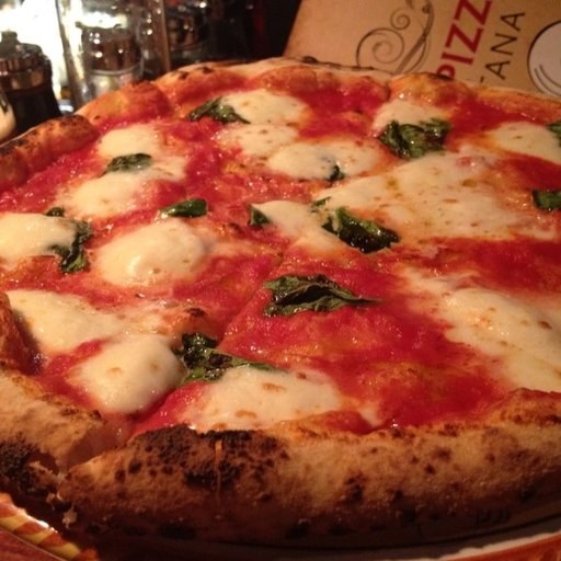
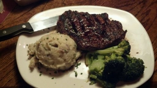
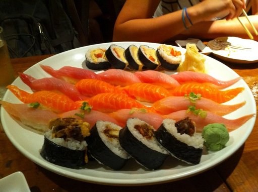
FoodVision Mini holds three classes: pizza, steak, and sushi. The archive unpacks into train/ and test/, each with one folder per class. The download runs once and is skipped if the directory already exists; the zip is removed after extraction. The counts are small enough to print in full.

Every total is a sum of the column above it: \(78+75+72=225\), \(25+19+31=75\), \(225+75=300\). Train shares: \(78/103=0.757\), \(75/94=0.798\), \(72/103=0.699\), \(225/300=0.750\).

Three facts follow from the table.

1. The split is 3:1 overall, but not exactly per class: steak keeps 79.8% for training, sushi only 69.9%. The test set is not a stratified copy of the train set, so per-class test scores carry different uncertainty.
2. The test set is 75 images, so one image is \(1/75 = 1.33\%\) of a per-image accuracy. A single flipped prediction moves the number by more than a percentage point.
3. With batch size 32, one training epoch has \(225 = 7 \times 32 + 1\), so 8 batches, the last holding one image. One test pass has \(75 = 2 \times 32 + 11\), so 3 batches, the last holding 11. Those short batches decide how accuracy is averaged in §8.

ImageFolder reads labels from the folder names in sorted order: pizza = 0, steak = 1, sushi = 2. It never reads a label file. Read dataset.classes instead of hardcoding the list; a class that appears in test but not train shifts the mapping, and a non-image file with a .jpg name crashes at load.

The photos are high-resolution colour images with varied backgrounds. The input pipeline squashes them to a fixed square, so the class signal has to survive the resize and the background.

4 · Preprocessing: make the input look like ImageNet

The pretrained weights are a function fitted to one kind of input. Change the input and the function no longer means what it meant. Four properties must match the weights.

IMAGENET_MEAN = [0.485, 0.456, 0.406]   # per channel, RGB
IMAGENET_STD  = [0.229, 0.224, 0.225]

train_tf = transforms.Compose([
    transforms.Resize((224, 224)),
    transforms.RandomHorizontalFlip(p=0.5),
    transforms.RandomRotation(degrees=10),
    transforms.ColorJitter(brightness=0.2, contrast=0.2, saturation=0.2, hue=0.1),
    transforms.ToTensor(),               # uint8 [0,255] HWC -> float [0,1] CHW
    transforms.Normalize(mean=IMAGENET_MEAN, std=IMAGENET_STD),
])

test_tf = transforms.Compose([
    transforms.Resize((224, 224)),
    transforms.ToTensor(),
    transforms.Normalize(mean=IMAGENET_MEAN, std=IMAGENET_STD),
])

Order is load-bearing: ToTensor makes the float tensor and moves channels first, then Normalize subtracts and divides per channel. Put Normalize first and it has no float tensor to act on.

4.1 · Why the mean and std must match

ToTensor maps a byte \(b \in [0,255]\) to \(b/255\), so a pixel is a number in [0, 1]. Normalize then computes, for each channel \(c\), \[ x'_c = \frac{x_c - \mu_c}{\sigma_c}. \] A mid-gray pixel \(x = 0.5\) becomes \((0.5-0.485)/0.229 = 0.066\) in red, \((0.5-0.456)/0.224 = 0.196\) in green, and \((0.5-0.406)/0.225 = 0.418\) in blue. The same gray turns into three different numbers because ImageNet's average photo is not neutral: its red channel is brighter than its blue. Across the [0, 1] input range, 0 maps to \(-2.12, -2.04, -1.80\) and 1 maps to \(2.25, 2.43, 2.64\). The network's inputs live around zero at unit scale, not in [0, 1].

Why the exact values matter: the first convolution computes \(z = \sum_c W_c x'_c + b\). Its weights \(W\) were learned while \(x'\) was the normalized value. Feed the raw pixel \(x\) instead. Since \(x_c = \sigma_c x'_c + \mu_c\), the filter sees \[ \sum_c W_c x_c = \sum_c \sigma_c W_c x'_c + \sum_c \mu_c W_c. \] The signal the filter sees is scaled by \(\sigma_c \approx 0.225\) — about 4.4× too small — and shifted by a constant \(\sum_c \mu_c W_c\) that differs for every filter. Every threshold the next layer learned now sits in the wrong place. Double normalization fails the same way in reverse: the response is scaled by \(1/\sigma_c\) and shifted the other way.

These statistics are part of the model's input contract, not a property of your food images. Recomputing the mean and std on the 225 training images would move the input to a distribution the weights never saw. Use the pretrained values even when your images are darker or more saturated than ImageNet's.

4.2 · Augmentation on train, none on test

The training pipeline adds three random transforms: a horizontal flip with probability 0.5, a rotation between \(-10°\) and \(10°\), and colour jitter on brightness, contrast, saturation and hue. The resize is fixed. The random transforms change the input on purpose while the label stays the same, so the head cannot memorise one appearance of each image. The test pipeline has none of them, so every epoch measures the same function on the same pixels.

Two details of the exact recipe. First, the values match the pretrained weights but the geometry is a shortcut: the code above resizes straight to 224×224 and squashes a non-square photo, while the weights' own transform resizes the short side to 256 and then center-crops 224, keeping the aspect ratio and discarding the edges. Ask the weights for the exact recipe:

weights = torchvision.models.EfficientNet_B0_Weights.DEFAULT
weights.transforms()
# ImageClassification(crop_size=[224], resize_size=[256],
#   mean=[0.485, 0.456, 0.406], std=[0.229, 0.224, 0.225],
#   interpolation=BICUBIC)

Both pipelines produce a 224×224 tensor; they do not produce the same pixels. Match the values exactly, and decide the geometry on purpose.

Second, ImageFolder stores file paths and applies the transform on access, so the dataset does not hold 225 decoded tensors in memory. The DataLoader builds batches of shape \((32, 3, 224, 224)\), shuffling the training set and leaving the test set in order so metrics compare across epochs.

5 · The model: EfficientNet-B0 and the head swap

EfficientNet-B0 (Tan and Le, 2019) comes from torchvision.models with weights trained on ImageNet. Load the best available weights and the model arrives in three parts.

Where the shapes come from: the 224×224 input is halved five times, \(224 \to 112 \to 56 \to 28 \to 14 \to 7\). The first convolution strides by 2, and four further stages halve the map again. The body ends with 1,280 feature maps of size \(7 \times 7\), which is \(1280 \times 49 = 62{,}720\) numbers per image. The average pool replaces each map with its mean, so the classifier reads 1,280 numbers whatever the spatial size. The old linear layer holds \(1280 \times 1000 + 1000 = 1{,}281{,}000\) parameters, and the total is \(4{,}007{,}548 + 1{,}281{,}000 = 5{,}288{,}548\).

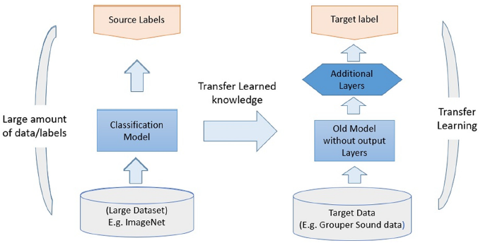
The head swap is one assignment:

model.classifier = nn.Sequential(
    nn.Dropout(p=0.2, inplace=True),
    nn.Linear(in_features=1280, out_features=3, bias=True),
).to(device)

The body is untouched. The new head reads the same 1,280 numbers and writes three logits: one for pizza, one for steak, one for sushi.

Count the new head. One output neuron reads all 1,280 features and holds 1,280 weights. Three outputs hold \(3 \times 1280 = 3{,}840\) weights, and each output carries its own bias: \(3\) more. So the head holds \[ 1280 \times 3 + 3 = 3840 + 3 = 3{,}843 \] parameters. With bias=False it would hold 3,840. The old head held 1,281,000, so the swap removes \(1{,}281{,}000 - 3{,}843 = 1{,}277{,}157\) parameters and the model falls from 5,288,548 to \(4{,}007{,}548 + 3{,}843 = 4{,}011{,}391\).

The contrast that matters is against the body. The new head is \(3{,}843 / 4{,}011{,}391 = 0.000958\), which is 0.096% of the model, about 1 parameter in 1,044. The old head was 333× larger than the new one. In data terms, the body holds one training image for every 17,811 of its parameters; the head holds one image for every 17.1 of its. The head is sized to the data; the body is not trained at all.

6 · Freeze, then count what can learn

Freezing is one attribute per parameter. requires_grad = False tells autograd not to record that parameter for a gradient. The forward pass still uses it, the backward pass leaves its .grad as None, and the optimizer has nothing to step.

for p in model.features.parameters():
    p.requires_grad = False

trainable = [p for p in model.parameters() if p.requires_grad]
print(len(trainable))                      # 2  (the linear weight and bias)
print(sum(p.numel() for p in trainable))   # 3843

Two tensors hold all 3,843 numbers: the \(3 \times 1280\) weight matrix and the 3-element bias. Dropout learns nothing.

Build the optimizer over every parameter, as the run does:

optimizer = torch.optim.Adam(model.parameters(), lr=1e-3)

This is safe: frozen parameters have no gradient, so Adam skips them. A tighter version passes trainable instead. Both update 3,843 numbers. The optimizer's argument list does not freeze the body; requires_grad does.

That distinction has teeth. If you pass only the head to the optimizer but forget requires_grad = False, the body still computes gradients on every backward pass — wasted work — and its batch-normalization statistics still change. Freezing removes the gradient; the optimizer list only removes the update.

One more thing freeze does not stop: batch normalization. Every batch-norm layer inside features carries running mean and variance buffers. requires_grad = False does not touch them. While the model is in training mode, each forward pass updates those buffers from the food batch, so the body's normalization drifts even though its weights do not. If you want the body fixed bit for bit, put the features in eval mode after the model's own train switch:

model.train()            # classifier dropout on, batch-norm in training mode
model.features.eval()    # body batch-norm now uses its stored ImageNet statistics

"Frozen" in PyTorch means "no gradient", not "no change".

7 · Three experiments that do not crash

The rules above are easy to agree with and easy to break. Each experiment asks for a prediction before the code. Write the prediction down. The paragraph after each block is the check.

7.1 · What happens when the input is 0–255 or BGR?

Predict first. The same pizza photo goes through three pipelines: the weights' own transform, one that feeds bytes from 0 to 255 with no normalization, and one that swaps red and blue. Which runs raise an error? Which still return the class "pizza"?

import torch, torchvision
from torchvision import transforms
from PIL import Image

weights = torchvision.models.EfficientNet_B0_Weights.DEFAULT
model = torchvision.models.efficientnet_b0(weights=weights).eval()
cats = weights.meta["categories"]
pizza = cats.index("pizza")

img = Image.open("../img/food-pizza.jpg").convert("RGB")
good = weights.transforms()(img).unsqueeze(0)
raw = transforms.Compose([transforms.Resize((224, 224)), transforms.ToTensor()])(img).unsqueeze(0) * 255
bgr = good[:, [2, 1, 0]]

with torch.inference_mode():
    for name, x in [("normalized", good), ("0-255", raw), ("BGR", bgr)]:
        p = model(x).softmax(1)[0]
        top = p.argmax().item()
        print(f"{name:10s} top={cats[top]:12s} p={p[top].item():.3f} pizza={p[pizza].item():.3f}")

Run from courses/dl-gen-ai/lessons, the folder that holds this page, so ../img/food-pizza.jpg resolves; the first call downloads the 20.5 MB weights once.

What happens. All three runs finish. No shape error, no warning, no NaN:

normalized top=pizza        p=0.578 pizza=0.578
0-255      top=hand blower  p=1.000 pizza=0.000
BGR        top=bakery       p=0.046 pizza=0.040

The normalized pipeline calls the photo pizza with probability 0.578. The byte pipeline is certain it is a hand blower. The BGR pipeline puts bakery first and drops pizza to 0.040, about 15 times below the normalized score. The tensor has the right shape and dtype in every case, so the forward pass cannot tell you the input is wrong. The rule: the input must match the weights in scale, channel order, and per-channel statistics; a legal tensor is not a correct tensor.

7.2 · What happens when the 1,000-class head stays?

Predict first. You freeze the body, keep the original 1,000-output classifier, and pass labels 0, 1, 2 for pizza, steak, sushi. Does CrossEntropyLoss reject a label that is smaller than the output size? What is the loss when every logit is zero, against 1.0986 for three classes?

import torch, torch.nn as nn

logits = torch.zeros(1, 1000, requires_grad=True)
loss = nn.CrossEntropyLoss()(logits, torch.tensor([0]))
print(round(loss.item(), 4))                    # 6.9078
loss.backward()
print(round(logits.grad[0, 0].item(), 3))       # -0.999
print(round(logits.grad[0, 500].item(), 3))     # 0.001
print(round(nn.CrossEntropyLoss()(torch.zeros(1, 3), torch.tensor([0])).item(), 4))  # 1.0986

What happens. No error. The loss is 6.9078, which is \(\ln 1000\), not the \(\ln 3 = 1.0986\) a three-class head would give. The gradient is -0.999 on the row for class 0 and +0.001 on each of the other 999 rows. Every step raises the three logits you use as labels and pushes the other 997 down. Training can still drive the loss down, because an argmax over 1,000 outputs can return 0, 1, or 2. But the head holds \(1280 \times 1000 + 1000 = 1{,}281{,}000\) parameters to make three decisions, and it starts from the loss of a 1,000-way problem. The rule: the output width must equal the number of labels you have, not merely contain them.

7.3 · What happens when you unfreeze the body at the head's learning rate?

Predict first. A two-input linear body has known weights. One Adam step at lr=1e-3. With the body frozen, how far does a body weight move? With the body unfrozen, how far does it move?

import torch, torch.nn as nn

def one_step(freeze):
    body = nn.Linear(2, 2, bias=False)
    with torch.no_grad():
        body.weight.copy_(torch.eye(2))
    if freeze:
        for p in body.parameters():
            p.requires_grad = False
    head = nn.Linear(2, 3)
    opt = torch.optim.Adam(list(body.parameters()) + list(head.parameters()), lr=1e-3)
    before = body.weight.detach().clone()
    loss = nn.CrossEntropyLoss()(head(body(torch.tensor([[1.0, 2.0]]))), torch.tensor([0]))
    opt.zero_grad()
    loss.backward()
    opt.step()
    return round((body.weight - before).abs().max().item(), 3)

print(one_step(freeze=True))    # 0.0
print(one_step(freeze=False))   # 0.001

What happens. The frozen body does not move: 0.0. The unfrozen body moves by 0.001, the full learning rate, on the first step. Adam normalises the first update by its own magnitude, so the step is the learning rate, not the gradient times the learning rate. On the real model with the body unfrozen, one backward pass fills .grad for all 4,007,548 body parameters. The risk is the direction: those weights were fitted to millions of ImageNet images, and one step from 225 food photos moves them toward a much smaller sample. The rule: a body that is allowed to learn needs its own, much smaller learning rate, and usually only its last blocks.

8 · Train and evaluate on 75 images

Cross-entropy loss on three logits, Adam at \(10^{-3}\), batch 32, five epochs. The whole run takes 16.181 seconds on a Tesla T4. The train step runs forward, loss, backward, and step in that order, with one change worth naming: only the head's gradients are non-None, so optimizer.step() moves nothing else.

model.train()
for X, y in train_dataloader:
    X, y = X.to(device), y.to(device)
    y_pred = model(X)                 # logits, shape (32, 3)
    loss = loss_fn(y_pred, y)         # nn.CrossEntropyLoss()
    optimizer.zero_grad()
    loss.backward()                   # fills .grad for the head only
    optimizer.step()
    batch_acc = (y_pred.argmax(dim=1) == y).float().mean()  # one batch accuracy, averaged below

The evaluation step calls model.eval() first and runs under torch.inference_mode(), which only turns autograd off.

model.eval()
with torch.inference_mode():
    for X, y in test_dataloader:
        logits = model(X.to(device))
        pred = logits.argmax(dim=1)

The five epochs produce this table.

Read the table in order. After one epoch the head is already at 73.39%, which is the body doing its job: the head started random and needed one epoch to map 1,280 features to three classes. Epoch 4 is the best: test loss 0.0963 and test accuracy 97.92%. Epoch 5 is slightly worse on both, so the last epoch is not the best one. The train accuracy is noisy — 98.05% at epoch 2, 84.38% at epoch 5 — and that is the metric, not the model forgetting: the train number is the mean of 8 batch accuracies, and the last batch holds one image. That single image is 1/8 of the epoch number, so right or wrong moves it by 12.5 points.

Say exactly what the accuracy is measured on. The reported test accuracy is the mean of three batch accuracies on 75 held-out images split 32 + 32 + 11. Each batch contributes 1/3 of the mean, so the 11-image batch weighs as much as a 32-image batch. One wrong image in the short batch costs \(1/11 \times 1/3 = 3.03\) points of the mean; one wrong image in a full batch costs \(1/32 \times 1/3 = 1.04\) points. A count of correct images would make one image worth \(1/75 = 1.33\) points instead.

The split is named test, but it is read at the end of every epoch. If you pick the best epoch by that number, 97.92% is a best-of-five on a check set, not a clean estimate on data the model never touched. Report the rule you used — "five epochs, last epoch" or "best epoch on the check set" — and do not call the best-of-five a held-out test score. If you want a per-image number under the same rule, count it directly:

correct, total = 0, 0
for X, y in test_dataloader:
    pred = model(X.to(device)).argmax(dim=1)
    correct += (pred == y).sum().item()
    total += y.numel()
print(correct / total)     # 0.0 .. 1.0, weighted by image, not by batch

The loss curves tell the same story: test loss falls from 0.5489 to 0.0963 by epoch 4, then rises to 0.1196, while test accuracy runs 73.4% → 97.9% → 95.8%. With 225 training images, do not read fine structure into a five-point curve.

The run also plots seven random test images with their true and predicted labels. That is a check on the pipeline — are the images upright, is the label order right, is the normalization undone correctly for display? — not a metric. A model can score well on those seven and still be wrong on the rest.

9 · What goes wrong

9.1 · Training the body on 225 images

Skip the freeze and loss.backward() fills .grad for all 4,007,548 body parameters. Adam at \(10^{-3}\) then takes a step on every one of them; §7.3 measures the size of one step on a two-weight toy. The body was fitted on millions of images, and 225 food photos can pull it away. Train accuracy can still climb, because the head is fitting the training set, while test accuracy can fall: the features that made the head work are no longer the ImageNet features. Fine-tuning is the controlled version: unfreeze a few later layers, use a much lower learning rate, and do it when you have more target data.

9.2 · Mismatching the normalization

Nothing crashes. Feed bytes from 0 to 255, channels in BGR order, or pixels that never met Normalize, and the forward pass runs on the wrong input. §7.1 shows the labels change; one forward pass cannot show whether the head recovers, so do not read that accuracy as a transfer result. Check one batch before training:

X, y = next(iter(train_dataloader))
print(X.shape, X.dtype)                  # torch.Size([32, 3, 224, 224]) torch.float32
print(X.min().item(), X.max().item())    # inspect; values depend on the images
print(X.mean(dim=(0, 2, 3)))             # descriptive, not a correctness test
print(X.std(dim=(0, 2, 3)))              # descriptive, not a correctness test

# Check the normalization operation with a pixel whose answer we know.
pixel = torch.full((3, 1, 1), 0.5)
mean = torch.tensor(IMAGENET_MEAN)[:, None, None]
std = torch.tensor(IMAGENET_STD)[:, None, None]
expected = (pixel - mean) / std
actual = transforms.Normalize(IMAGENET_MEAN, IMAGENET_STD)(pixel)
assert torch.allclose(actual, expected)
print(actual[:, 0, 0])                  # tensor([0.0655, 0.1964, 0.4178])

The subtraction and division use ImageNet's statistics, not this batch's. Consequently the food images need not have mean 0 or standard deviation 1 after normalization. Even a correctly normalized constant image has zero spatial standard deviation. A minimum of 0 alone proves nothing; inspect the transform chain and check a known pixel. To check RGB order, inspect a decoded image before normalization and compare its channel values.

9.3 · Forgetting requires_grad = False

The model runs; the only symptom is that the body changes. Check before the first step, and again after one backward pass:

print(sum(p.numel() for p in model.parameters() if p.requires_grad))  # 3843
model.features[0][0].weight.grad is None                              # True when frozen

If the first line prints 4,011,391, the freeze did not take. The count reads requires_grad directly; a summary can be a stale snapshot.

9.4 · Evaluating before eval()

model.eval() does two things: dropout stops zeroing features, and batch normalization uses its running statistics instead of the batch's. Skip it, and the prediction for one image depends on the other images in its batch, so the same weights give different test numbers on different runs. torch.inference_mode() only turns autograd off; it does not switch dropout or batch norm. Put model.eval() at the top of the test step and model.train() at the top of the train step.

9.5 · Two quiet ones

• The check set is read every epoch. Choose the best epoch by that number and it is a validation score. Carve a validation set out of the training images if you need a score on data the model never influenced.
• Batch-averaged accuracy is not per-image accuracy. With \(225 = 7 \times 32 + 1\) and \(75 = 2 \times 32 + 11\), the short last batch carries the same weight as a full one. Count correct images and divide by the total when the number will be compared across batch sizes.

Hands-on

1. Load efficientnet_b0(weights=EfficientNet_B0_Weights.DEFAULT). Predict the trainable count after you freeze model.features, then print sum(p.numel() for p in model.parameters() if p.requires_grad). Check 3,843 before you trust any summary line.
2. Inspect one training batch's shape, dtype, range, and channel statistics. Predict the shape and dtype of a full batch before you print them. Check (32, 3, 224, 224) and float32 for a full batch. Run the known-gray-pixel check in §9.2; explain why correctly normalized food images need not have zero channel means.
3. Train one epoch, then evaluate the same weights twice: once with model.eval() and once without. Predict which number will move, and why, before the second pass. Compare the two test accuracies and state which one the page would report.
4. Swap in Linear(1280, 3, bias=False) and count again: 3,840. Predict the count before you run it. Put the bias back. The difference is one number per class, and it is worth knowing where it comes from.

One-line understanding. Keep the 4,007,548 pretrained parameters that already see, and train the 3,843 parameters that name three foods — match the input to the weights, and freeze everything the weights already know.

References

• Tan, Le. EfficientNet: Rethinking Model Scaling for Convolutional Neural Networks (ICML 2019). arXiv:1905.11946 — the B0 body this page freezes, its 224×224 input, and the 1,280-channel feature vector.
• Deng et al. ImageNet: A Large-Scale Hierarchical Image Database (CVPR 2009). image-net.org paper — the 1,000 classes and the dataset whose per-channel statistics the weights expect.
• Yosinski, Clune, Bengio, Lipson. How transferable are features in deep neural networks? (NIPS 2014). arXiv:1411.1792 — evidence that early-layer features transfer and later layers are more task-specific.