Trace U-Net down and up, then score the mask with Dice

A classifier gives one answer per image. Segmentation gives one answer per pixel, so the output is a grid the same size as the photo. U-Net builds that grid by going down and then up. Going down makes the map small and full of meaning. Going up makes it large again, and the skips hand back the detail that going down destroyed.

flowchart LR
  IMG[image 512²] --> DOWN[down: what]
  DOWN --> BOT[bottom 32²]
  BOT --> UP[up: where]
  UP --> CAT[concat skips]
  CAT --> OUT[1×1 logits]
  OUT --> DICE[dice]

One rule fixes the order: resolution falls while the map learns what is present, then rises while the skips restore where it is.

1 · One answer per pixel

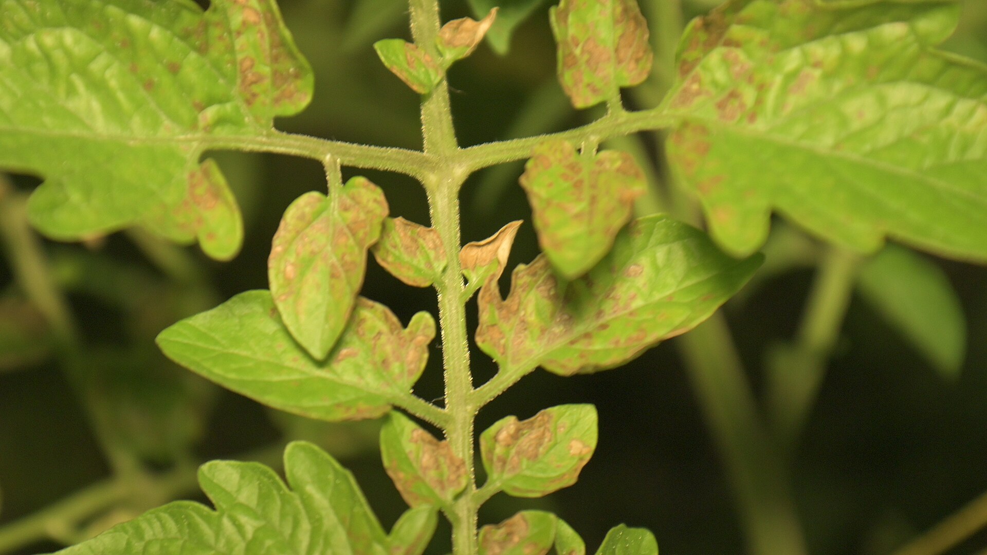
A classifier reads a 326×235 leaf photo and returns one score per class. A segmentation model returns one score at every pixel position. For this photo that is \(326 \times 235 = 76{,}610\) decisions, all in one grid.

That single change forces the architecture. A classifier may pool the whole image into one vector, so a lesion in the top-left and the same lesion in the bottom-right can give the same answer. A segmentation model may not. It must put the 1 on the pixels that carry the lesion and the 0 on the pixels that do not.

The target is called a mask. It is an image with one value per pixel: 1 on the foreground class, 0 on everything else. It has the same width and height as the photo, so position \((i,j)\) in the mask is position \((i,j)\) in the photo. That alignment is the contract. A mask shifted by one pixel teaches the model the wrong boundary.

With two classes, one output channel and a sigmoid per pixel is enough, because \(P(\text{background}) = 1 - P(\text{foreground})\). With \(C\) classes the last layer writes \(C\) channels at each position and a softmax runs across the channels. The U-Net paper introduced this shape for biomedical images, where the boundary between structures is the point: a tumour, a cell wall, a lesion. There the mask guides surgical planning and measures: count the 1s and you have the area. The same shape works for a leaf, because the disease is a region, not a label.

2 · The words this page uses

Seven groups of words carry the rest of the page. Read them once. Each comes back with a toy number later.

2.1 · Image, pixel, channel, mask

A pixel is one position in the grid. A channel is one number per position: an RGB image has three, a feature map has as many as the layer writes. A torch batch is (N, C, H, W), so four colour images at 512×512 are (4, 3, 512, 512). A mask is the target grid: 1 on the foreground, 0 on the background, same H and W as the photo.

2.2 · Kernel, stride, padding, feature map

A kernel (or filter) is a small grid of weights, 3×3 here. It slides over the input; at each position it multiplies the patch under it by its weights and adds the products into one number. A feature map is the grid of those numbers. One kernel writes one channel, so 64 kernels write 64 channels.

Stride is how far the kernel moves per step. Stride 1 moves one pixel. Stride 2 moves two, so the output is half as wide and half as tall. Padding is a ring of zeros around the border, so the kernel can centre on an edge pixel. Padding 1 with a 3×3 kernel keeps H and W unchanged.

The receptive field is the patch of the input that one output cell can see. Two 3×3 convolutions in a row see 5×5, because the second combines three outputs of the first, and each of those already saw 3×3. Every extra 3×3 adds one pixel of reach on each side.

2.3 · Downsampling and max pooling

Downsampling is any operation that makes H and W smaller. Max pooling takes the largest value in each 2×2 block. A 2×2 pool with stride 2 halves both sides. It keeps the strongest response and drops the exact position inside the block. The pool has no weights: it is a fixed rule, and training cannot change it.

2.4 · Upsampling and transposed convolution

Upsampling is any operation that makes H and W larger. Nearest neighbour copies each value into a 2×2 block: a fixed rule, no weights. A transposed convolution (also called up-convolution, sometimes deconvolution) runs the shape backwards: with kernel 2 and stride 2, each input value writes a 2×2 patch of output, and the weights are learned. The name deconvolution is a misnomer; it does not undo a convolution, it only reverses the shape.

2.5 · Contracting path, expansive path, bottleneck

The contracting path (encoder) is the down half: convolution blocks plus pools. It trades resolution for context. The map shrinks, the channels grow, and each cell covers more of the photo. The bottleneck is the smallest map at the bottom: 1024 channels at 32×32. It holds the most meaning and the least position. The expansive path (decoder) is the up half: up-convolutions plus convolution blocks. It trades context back for resolution.

2.6 · Skip connection and concatenation

A skip connection is a wire that carries an encoder map straight across to the decoder at the same resolution. Concatenation joins two maps along the channel axis: 512 channels plus 512 channels gives 1024 channels, with H and W unchanged. In U-Net the skip is a concat. In a ResNet the shortcut is an add, and §4 says why the difference matters.

2.7 · Logit, sigmoid, threshold

A logit is the raw score the last layer writes; it can be any real number. Sigmoid, \(\sigma(z) = 1/(1+e^{-z})\), squashes a logit into the range 0 to 1, so it reads as a probability. A threshold compares that probability with 0.5 to produce the 0/1 mask.

3 · Down, bottom, up

U-Net goes down and up. That is the name: the down half and the up half make a U. This section walks the shape once, with the channel counts of the code.

3.1 · Going down: a double conv, then a pool

Each encoder stage is a double conv: 3×3 convolution with padding 1, BatchNorm, ReLU, then the same again. Padding 1 keeps the size, so the block changes only the channel count. A 2×2 max pool with stride 2 then halves both sides. The first block lifts the 3 colour channels to 64; every later block doubles, 64 → 128 → 256 → 512 → 1024. The sides halve at every pool: 512 → 256 → 128 → 64 → 32.

At the bottom, one cell stands for a 16×16 block of the input, because \(512/32 = 16\). The map knows a lot about what is there (1024 channels) and little about where: one cell covers \(16 \times 16 = 256\) input pixels. That is the information the decoder has to put back: the localization.

3.2 · The whole ladder in one table

Channels first, spatial size second. The batch dimension rides along unchanged, so (4,3,512,512) becomes (4,1024,32,32) at the bottom and (4,1,512,512) at the output.

3.3 · Going up, and the swap

Each decoder stage starts with a 2×2 transposed convolution with stride 2. It doubles the map and halves the channels: 1024 at 32×32 becomes 512 at 64×64. Then the skip concatenates the matching encoder map, and a double conv mixes the two groups. Four stages take 32×32 back to 512×512, and a 1×1 convolution writes one logit per pixel.

Here is the swap the name hides. Going down, a pool halves the map: a fixed rule with no weights. Going up, a convolution doubles it: a learned rule with weights. The up path does not stretch the bottleneck with an interpolation. It runs a convolution that decides what to write into the new, higher-resolution cells. That is how the coarse evidence at the bottom reaches the fine grid at the top.

Many implementations use nn.Upsample(scale_factor=2) followed by a normal 3×3 conv instead of nn.ConvTranspose2d. The idea is the same: enlarge the map, then let a convolution decide the values. The notebook uses the transposed convolution, which does the resize and the mixing in one layer.

4 · Why concatenate, not add

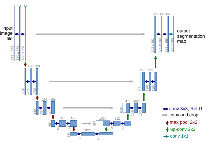
At the first skip both maps are 512 channels at 64×64, so an elementwise add would run. The shapes are not the reason the code concatenates.

The encoder's 512 channels carry fine detail: edges, texture, the exact boundary of a spot. The decoder's 512 channels carry coarse evidence: "this region is diseased", built from the 32×32 bottom. Adding channel \(i\) of one to channel \(i\) of the other forces two different measurements into one number, and the next layer cannot tell them apart again. Concatenating keeps the two groups side by side: 1024 channels, same positions, different meanings. The next 3×3 conv learns which group to trust where.

A ResNet block adds because its shortcut carries the same quantity the block is refining: \(H(x) = F(x) + x\), and the identity is meaningful. A U-Net skip carries a different, finer measurement. Addition needs equal shapes and a shared channel meaning; concatenation needs only equal height and width, and it keeps the detail separate.

5 · The arithmetic on a toy grid

Every number here is small enough to check by hand. The same operations run at 512×512; only the count changes.

5.1 · A 3×3 kernel on a 4×4 grid

Take this input and a kernel of nine ones, stride 1, no padding:

The kernel sits on the top-left 3×3 patch: \(1+2+3+5+6+7+9+10+11 = 54\). Move one column right: \(2+3+4+6+7+8+10+11+12 = 63\). Move one row down: \(5+6+7+9+10+11+13+14+15 = 90\). Bottom-right: \(6+7+8+10+11+12+14+15+16 = 99\). The output is

Why 2×2? A 3-wide kernel has only two positions to start in a 4-wide input. The rule is output side \(= 4 - 3 + 1 = 2\). Change the kernel to a vertical-edge detector and the same slide reports the step where the image goes from dark to bright. The slide does not change; the weights decide what it looks for.

5.2 · Padding keeps the size

Without padding, every 3×3 conv shaves one pixel off each side, and the mask would stop matching the photo. Padding 1 adds a ring of zeros. The top-left output cell of the 4×4 toy now covers \(1+2+5+6 = 14\), because the other five cells of its window are zeros. The output is 4×4 again: \[ \text{side} = \frac{\text{input} + 2 \cdot \text{padding} - \text{kernel}}{\text{stride}} + 1 = \frac{4 + 2 - 3}{1} + 1 = 4. \] Read the formula once; after this page, the shape table is faster.

5.3 · A pool halves the map

Take this 4×4 input. A 2×2 max pool with stride 2 reads four blocks and keeps the largest value in each.

The first block is 1, 3, 5, 6, so max gives 6 and average gives 3.75. Max keeps the strongest response; average keeps the mean. U-Net uses max. The pool has no weights and the exact position inside each block is gone. That loss is what the skip repairs.

5.4 · An up-convolution doubles it back

Take a 2×2 input, a 2×2 kernel of ones, and stride 2. Each input value writes a 2×2 block of itself into the output: 1 goes top-left, 2 top-right, 3 bottom-left, 4 bottom-right.

That is nearest-neighbour upsampling, because the weights are all ones. The weights are parameters, so training can change what each value writes. In the network the input has 1024 channels and the output 512, so each output value is a weighted sum of 1024 numbers, not a copy of one. The size rule is output \(= (\text{input} - 1) \cdot \text{stride} + \text{kernel} = (2 - 1) \cdot 2 + 2 = 4\). For the real map: \((32 - 1) \cdot 2 + 2 = 64\).

With kernel 3 and stride 2 the blocks overlap and the overlaps add. That is how a transposed convolution can blend neighbours instead of copying them.

5.5 · Concat, channels, parameters

At the first skip, the up-conv writes 512 channels at 64×64 and the encoder map has 512 at 64×64. The concat gives 1024 at 64×64, and the double conv reads 1024 and writes 512.

Count the first encoder block. Conv 1 reads 3 channels and writes 64: \(9 \times 3 \times 64 = 1{,}728\) weights plus 64 biases. BatchNorm adds two parameters per channel, \(2 \times 64 = 128\). Conv 2 reads 64 and writes 64: \(9 \times 64 \times 64 = 36{,}864\) weights plus 64 biases, plus another 128 for BatchNorm. The total is \(1{,}728 + 64 + 128 + 36{,}864 + 64 + 128 = 38{,}976\).

The first decoder block is the expensive one because the concat doubled its input. Conv 1 reads 1024 and writes 512: \(9 \times 1024 \times 512 + 512 = 4{,}719{,}104\), plus \(2 \times 512 = 1{,}024\) for BatchNorm. Conv 2 reads 512 and writes 512: \(9 \times 512 \times 512 + 512 = 2{,}359{,}808\), plus 1,024. The total is \(7{,}080{,}960\), about 180 times the first encoder block.

At four bytes per parameter, \(31{,}043{,}521 \times 4 = 124{,}174{,}084\) bytes, about the 124 MB checkpoint the run loads.

6 · Loss and Dice: the number that trains and the number that judges

6.1 · Binary cross-entropy on a logit

The model writes one raw score per pixel, \(z\). For a target \(y\) of 0 or 1, the loss at that pixel is \[ \ell(z,y) = -\left[y \log \sigma(z) + (1-y)\log(1-\sigma(z))\right]. \] In words: if the target is 1, the loss is minus the log of the predicted probability of 1; if the target is 0, it is minus the log of the predicted probability of 0. A confident correct answer costs almost nothing. A confident wrong answer costs a lot.

At z = 0 the model is unsure and pays ln 2 = 0.6931 whatever the label. A confident correct logit pays 0.1269; a confident wrong one pays 2.1269.

BCEWithLogitsLoss takes the raw logit and applies the sigmoid inside, in a stable way. Do not apply sigmoid first: that squashes the value twice and shrinks the gradient.

6.2 · Dice by hand

Dice measures overlap, not per-pixel error: \[ D = \frac{2|P \cap G|}{|P| + |G|} = \frac{2\,\mathrm{TP}}{2\,\mathrm{TP} + \mathrm{FP} + \mathrm{FN}}. \] The second form follows from \(|P| = \mathrm{TP} + \mathrm{FP}\) and \(|G| = \mathrm{TP} + \mathrm{FN}\).

A 4×4 toy. Ground truth \(G\) has five lesion pixels; prediction \(P\) has four. Read the grids row by row:

Count the overlap. Three predicted pixels sit on a true lesion, so \(\mathrm{TP} = 3\). One predicted pixel sits on a 0 in the truth, so \(\mathrm{FP} = 1\). Two lesions are missed, so \(\mathrm{FN} = 2\). The prediction has \(3 + 1 = 4\) positives; the truth has \(3 + 2 = 5\). Dice is \[ D = \frac{2 \times 3}{4 + 5} = \frac{6}{9} = 0.667. \]

6.3 · The accuracy trap

Now predict 0 everywhere on the same grid. The mask has \(16 - 5 = 11\) background pixels, so accuracy is \(11/16 = 0.6875\). Dice is 0, because the prediction has no positive pixel to overlap. A sparse target makes a do-nothing model look about 69% correct. Dice ignores the 11 true negatives that accuracy rewards, which is why the run reports Dice.

The code's Dice is a batch-level score. It thresholds each sigmoid at 0.5, then sums the intersection and both masks over the four images. A large lesion therefore contributes more than a small one; a per-image mean would weight each leaf equally. The epsilon \(10^{-7}\) guards the 0/0 case: when both masks are empty, the same epsilon sits above and below the line, so the function returns 1, not 0. Read that edge case before you trust a score.

def dice_score(preds, labels, eps=1e-7):
    preds = (preds.sigmoid() > 0.5).float()
    intersection = (preds * labels).sum()
    return (2 * intersection + eps) / (preds.sum() + labels.sum() + eps)

This is the code's function in four lines. It returns one number for the whole batch, not one per image.

Dice can also be a loss: \(1 - D\) on soft probabilities is differentiable and pushes the overlap up directly. This run does not do that. It trains on BCE and reports Dice, so the two numbers answer different questions: BCE trains each pixel, Dice judges the region.

7 · The data: the target must match the photo

7.1 · Pairs, paths, sort order

kagglehub.dataset_download caches the archive and returns the local path. The archive holds 588 images and 588 masks in two directories. It unpacks into a nested data/data folder, so the paths read data/data/images and data/data/masks. The doubled name is the archive's structure, not a typo.

The two filename lists are sorted and paired by index: image \(i\) with mask \(i\). Sorting is not cosmetic. If one list sorts differently, every target attaches to the wrong photo, and the loss can still fall while the model learns nothing useful.

7.2 · Mask values and the channel

The image is JPEG, RGB, 326 wide and 235 high, uint8. The mask is PNG, the same size, uint8, and its foreground may be stored as 255. PNG is lossless, so the mask's values survive the file. JPEG compression would blur the boundary and create values that are neither 0 nor 1. The code binarizes it: mask[mask != 0] = 1.

The mask then gets a channel dimension: (512, 512) becomes (1, 512, 512). One channel is enough for two classes because the probabilities sum to one: \(P(\text{background}) = 1 - P(\text{foreground})\). The model writes one logit per pixel, and sigmoid gives the foreground probability.

The dataset class is the whole pipeline for one sample: open the photo and the mask, binarize the mask, run the transform on both, put the channel back.

from torch.utils.data import Dataset
from PIL import Image
import numpy as np, os

class SegmentationDataset(Dataset):
    def __init__(self, img_list, mask_list, transform=None):
        self.img_list, self.mask_list, self.transform = img_list, mask_list, transform

    def __len__(self):
        return len(self.img_list)

    def __getitem__(self, i):
        img = np.array(Image.open(os.path.join(ROOTDIR.train, self.img_list[i])).convert("RGB"))
        mask = np.array(Image.open(os.path.join(ROOTDIR.train_mask, self.mask_list[i])).convert("L"))
        mask[mask != 0] = 1
        aug = self.transform(image=img, mask=mask)
        img, mask = aug["image"], aug["mask"]
        return img, mask.reshape(1, mask.shape[0], mask.shape[1])

One sample at a time; the DataLoader stacks four into a batch. The transform receives both arrays, so a flip hits the photo and the target together.

7.3 · Split and batches

The split takes 20% for validation. \(0.2 \times 588 = 117.6\), and the code truncates to 117. Training gets \(588 - 117 = 471\). At batch size 4, training has \(\lceil 471/4 \rceil = 118\) batches — 117 full batches of 4 plus one of 3 — and validation has \(\lceil 117/4 \rceil = 30\) batches — 29 full plus one of 1. Three epochs therefore run \(118 \times 3 = 354\) training batches and \(30 \times 3 = 90\) validation batches.

The validation split is the first 117 names in sorted order, not a random sample. If the filenames group leaves by session or condition, the validation score describes that group rather than the whole problem. Keep that in mind when you read the number. The notebook also fixes seed 123 for numpy and torch, so a rerun repeats the split and the augmentation draws.

7.4 · Transforms: same spatial change on both

Training resizes to 512×512, rotates by at most 15° with probability 0.1, flips horizontally with probability 0.5, normalizes, and converts to a tensor. Validation resizes, normalizes, and converts: no random step. Normalization with mean 0, std 1 and max_pixel_value=255 is just \(x/255\), which puts pixels in 0–1. The network starts from random weights, so there is no inherited normalization contract to match.

The same spatial transform must hit the image and the mask. A flip of the image without the mask turns the target into a mirror image of the truth. This is why the transform takes both in one call.

train_tf = A.Compose([
    A.Resize(512, 512),
    A.Rotate(limit=15, p=0.1),
    A.HorizontalFlip(p=0.5),
    A.Normalize(mean=(0, 0, 0), std=(1, 1, 1), max_pixel_value=255),
    ToTensorV2(),
])
val_tf = A.Compose([
    A.Resize(512, 512),
    A.Normalize(mean=(0, 0, 0), std=(1, 1, 1), max_pixel_value=255),
    ToTensorV2(),
])

A batch is (4, 3, 512, 512) images and (4, 1, 512, 512) masks. The mask channel is 1 because the task is binary.

8 · The code, and what happens when …

The real model is long. A small one carries the same wiring and runs in under a second, so this section builds the small one, walks its shapes, then breaks it on purpose. Each experiment asks for a prediction before the code. Write the prediction down; the paragraph after the code is the check.

8.1 · The building block

double_conv is used 9 times: five times going down, four times after each concat, and nowhere else. It changes channels and keeps H and W, because every convolution has padding 1.

def double_conv(cin, cout):
    return nn.Sequential(
        nn.Conv2d(cin, cout, 3, padding=1), nn.BatchNorm2d(cout), nn.ReLU(inplace=True),
        nn.Conv2d(cout, cout, 3, padding=1), nn.BatchNorm2d(cout), nn.ReLU(inplace=True),
    )

Read the two convs as "3×3, same size, new channel count", twice. The block never resizes a map.

8.2 · A tiny U-Net with the same wiring

Two down stages, a bottom, two up stages. Every channel count is small enough to follow. The wiring follows the real model, with 8 and 16 channels instead of 64 and 512.

import torch, torch.nn as nn

def block(cin, cout):
    return nn.Sequential(
        nn.Conv2d(cin, cout, 3, padding=1), nn.ReLU(),
        nn.Conv2d(cout, cout, 3, padding=1), nn.ReLU())

class TinyUNet(nn.Module):
    def __init__(self):
        super().__init__()
        self.d1 = block(3, 8);    self.d2 = block(8, 16)
        self.b  = block(16, 32)
        self.u2 = nn.ConvTranspose2d(32, 16, 2, 2)
        self.c2 = block(16 + 16, 16)
        self.u1 = nn.ConvTranspose2d(16, 8, 2, 2)
        self.c1 = block(8 + 8, 8)
        self.out = nn.Conv2d(8, 1, 1)
        self.pool = nn.MaxPool2d(2, 2)

    def forward(self, x):
        x1 = self.d1(x)                      # (1, 8, 64, 64)
        x2 = self.d2(self.pool(x1))          # (1, 16, 32, 32)
        b  = self.b(self.pool(x2))           # (1, 32, 16, 16)
        d2 = self.u2(b)                      # up: (1, 16, 32, 32)
        d2 = self.c2(torch.cat([x2, d2], 1)) # concat: 16 + 16 -> 16
        d1 = self.u1(d2)                     # up: (1, 8, 64, 64)
        d1 = self.c1(torch.cat([x1, d1], 1)) # concat: 8 + 8 -> 8
        return self.out(d1)                  # (1, 1, 64, 64)

29,465 parameters. The real model has 31,043,521, mostly because its channel counts are much larger.

8.3 · Walk the shapes

Predict first. A (1, 3, 64, 64) image goes in. What comes out, and what is the channel count at the bottom?

m = TinyUNet()
x = torch.zeros(1, 3, 64, 64)
print(m(x).shape)          # torch.Size([1, 1, 64, 64])

x1 = m.d1(x); x2 = m.d2(m.pool(x1)); b = m.b(m.pool(x2))
print(x1.shape, x2.shape, b.shape)
# torch.Size([1, 8, 64, 64]) torch.Size([1, 16, 32, 32]) torch.Size([1, 32, 16, 16])

The output has the input's height and width. That is the contract of segmentation: one score for every input pixel.

The real model adds BatchNorm and four stages, and its bottom is 1024 channels at 32×32. Its 1×1 conv reads 64 channels and writes 1. Nothing else changes.

8.4 · What happens when you remove a skip?

Predict first. The up-conv writes 16 channels at 32×32. The skip would add another 16. Drop the skip: what does c2 receive, and what does it expect?

class NoSkip(TinyUNet):
    def forward(self, x):
        x1 = self.d1(x)
        x2 = self.d2(self.pool(x1))
        b  = self.b(self.pool(x2))
        d2 = self.c2(self.u2(b))              # no concat
        d1 = self.c1(torch.cat([x1, self.u1(d2)], 1))
        return self.out(d1)

What happens. RuntimeError: expected input[1, 16, 32, 32] to have 32 channels, but got 16 channels instead. The concat is not decoration; it is the shape contract c2 is built on. Rebuild c2 as block(16, 16) and the model runs with 27,161 parameters, working from the bottleneck alone. That is a different, coarser model: the decoder no longer receives the mid-level encoder map.

8.5 · What happens when you add instead of concatenate?

Predict first. The up-conv writes 16 channels and the encoder map has 16, so an add is legal. Does the next block run?

d2 = self.c2(self.u2(b) + x2)   # add, not cat

What happens. The add runs and still has 16 channels. c2 expects 32, so you get the same RuntimeError. Rebuild c2 as block(16, 16) and it runs with 27,161 parameters, 2,304 fewer than the concat model. Nothing crashes. The encoder's edge map is now summed into the decoder's coarse map, so the network can no longer keep the two apart. The parameter count barely moves; the lost information is the cost, and no error warns you.

8.6 · What happens when the mask keeps 255?

Predict first. A mask straight from the PNG has 255 on the lesion. At logit 0, what loss does BCEWithLogitsLoss return for that pixel, and what gradient does it send?

z = torch.zeros(1, 1, 1, 1, requires_grad=True)
loss = nn.BCEWithLogitsLoss()(z, torch.ones(1, 1, 1, 1) * 255)
print(loss.item())      # 0.6931
loss.backward()
print(z.grad.item())    # -254.5

What happens. The loss looks normal: 0.6931 is the same value a 0/1 target gives at logit 0. But the gradient is −254.5 instead of −0.5. The 255 and the \(1 - 255\) terms nearly cancel in the loss, so the number hides the bug; the gradient does not. One step moves the weights about 500 times too far. Binarize before the loss.

8.7 · What happens when validation gets the training transform?

Predict first. The notebook builds val_dataset with train_transform. What changes in the validation score?

val_dataset = SegmentationDataset(val_images_list, val_masks_list, transform=val_transform)
# the run passes train_transform here

What happens. With the training transform, each validation image gets a random rotation or flip on every pass. The score now depends on which random draws that epoch produced, so two epochs are not measured on the same data. The fix is one word: val_transform. Validation is for comparison, so it must be deterministic.

8.8 · What happens when the input is not divisible by 16?

At 512 the four pools divide exactly, so every upsampled map matches its skip. At the original 235-pixel height the chain is 235 → 117 → 58 → 29 → 14, and doubling gives 28, 56, 112, 224 — short of 29, 58, 117, 235. The concat would fail. The code's padder copies the smaller map into the top-left of a zero tensor the size of the encoder map. Resizing to 512 avoids the mismatch, but the padder stays for other sizes.

9 · The run: 31M parameters, 3 epochs, Dice 0.25

9.1 · The numbers

The run uses 31,043,521 parameters, Adam at \(3 \times 10^{-3}\), batch size 4, and 3 epochs. The loss is BCEWithLogitsLoss. Each epoch runs 118 training batches and 30 validation batches. The model and each batch go on the GPU when one is available. Training sets model.train(); validation sets model.eval() and runs under torch.no_grad(), so BatchNorm uses its running statistics and no graph is built.

Read the validation column first. Loss falls from 1.7567 to 1.5315, a drop of 0.2252, and Dice rises from 0.1897 to 0.2502, a gain of 0.0605. The model is learning, but a Dice of 0.25 is a poor overlap. The training Dice bounces — 0.2987, 0.2627, 0.3525 — and ends \(0.3525 - 0.2502 = 0.1023\) above validation. Three epochs are too few to call that overfitting; the run is still underfit.

9.2 · The printed loss is four times the mean

One training step is five lines in a fixed order:

pred = model(img)                  # forward
loss = criterion(pred, mask)       # BCE on the raw logits
optimizer.zero_grad()              # clear the last step
loss.backward()                    # gradients
optimizer.step()                   # update the weights
running_loss += loss.item() * 4    # the x4, one batch

Swap zero_grad and step and the gradients accumulate across batches. The order is the contract.

The loop adds loss.item() * 4 for each batch, then divides by the number of batches. Each batch mean is counted four times, so the printed number is about four times the per-pixel mean. Divide by 4 to compare with \(\ln 2 = 0.6931\), the loss of a constant 0.5 predictor: \(1.4592/4 = 0.3648\) at epoch 1, \(1.5315/4 = 0.3829\) at epoch 3. The Dice column is not scaled.

9.3 · The checkpoint is not the run

The inference section loads a separate 124 MB checkpoint, downloaded with gdown, not the 3-epoch weights. It scores 0.7050 Dice on the first validation image. That number is a single-image overlap from different weights. It is not the validation mean, and it is not evidence that the model generalizes. The 3-epoch validation mean is 0.2502.

The run saves its state_dict to unet_scratch_new.pth; inference loads unet_scratch.pth. They are not the same weights.

Two details in that inference cell are easy to miss. It thresholds the raw logit at 0 rather than the probability at 0.5; the two cuts agree because sigmoid is increasing and \(\sigma(0) = 0.5\). And it opens the photo with cv2.imread, which returns BGR, while training used PIL and RGB. Convert with cv2.cvtColor(img, cv2.COLOR_BGR2RGB), or the model sees the channels swapped.

9.4 · What Dice proves, and what it does not

A Dice score proves overlap on the pixels it measured. It does not prove the boundary is in the right place: Dice counts pixels, not distance, so a mask that covers the lesion plus a one-pixel ring loses only the ring's share. It does not prove the model found the disease for the right reason, and one image says little about a new farm, camera, or leaf. The validation split is the first 117 sorted filenames, so even the validation mean describes that group.

For scale, Dice 0.7050 corresponds to IoU \(0.7050/(2 - 0.7050) = 0.5444\) when the two masks have the same size. The conversion is \(\mathrm{IoU} = D/(2-D)\); it assumes equal mask sizes, so treat it as a rough reading, not a second measurement.

Hands-on

1. Plot one training image and its mask side by side before you train. Check that the lesion in the photo is the white region in the mask, and that the two are aligned.
2. Draw the 2×2 up-conv on paper: input 1, 2, 3, 4, kernel all ones, stride 2. Check the 4×4 in §5.4. Then set the top-right weight to 0.5 and recompute the top row. Confirm with the code.
3. Run TinyUNet and print every shape in the forward pass. Then remove one skip and read the error. Write the channel count it expected and the one it got.
4. Compute the first encoder block's 38,976 parameters and the first decoder block's 7,080,960 with the arithmetic in §5.5. Add the four group totals and check 31,043,521. Say which single choice makes the decoder block expensive.
5. Run the four-line Dice function on the 4×4 tensors. Check 0.667. Then set the prediction to all zeros and check 0 and 0.6875 accuracy.
6. Run the 255-target loss. Print the loss and the gradient. Explain why the loss looks normal and the gradient does not.

One-line understanding. U-Net goes down to learn what is there and up to say where; the skips carry the fine maps the pool destroyed, and Dice — not pixel accuracy — tells you whether the overlap is real.

References

• Ronneberger, Fischer, Brox. U-Net: Convolutional Networks for Biomedical Image Segmentation (MICCAI 2015). arXiv:1505.04597 — the encoder-decoder, the skip connections, and the original biomedical task.
• Leaf Disease Segmentation Dataset. kaggle.com/datasets/fakhrealam9537/leaf-disease-segmentation-dataset — the 588 image-mask pairs used here.
• Dice, L. R. Measures of the Amount of Ecologic Association Between Species (1945). doi:10.2307/1932409 — the overlap coefficient the score is named for.